- How to use “real” UART
- Arduino’s Automatic Reset
- Linux always toggles DTR & RTS
- Espressif’s Automatic Reset
- Talking to Espressif’s Bootloader
- The ESP32-S2 reset pin
- Reproducing Espressif’s reset circuit
- The missing part of Espressif’s reset circuit
- Transistors in reverse and redundant circuits
- The serial TX path seems to be down
The mystery
In the previous article, I briefly mentioned a slight difference between the ESP-Prog and the reproduced circuit, when it comes to EN:


Focusing on EN, it looks like the voltage level goes back to 3.3V much faster on the ESP-Prog than on the breadboard circuit. The grid is horizontally spaced at 2ms, so it takes about 0.8ms for the breadboard circuit to cross 2V, and about 0.2ms for the ESP-Prog.
Zooming in
I actually noticed this when observing the behavior of the breadboard circuit with my oscilloscope when trigering a reboot into bootloader mode. This uses the same C program as the one at the end of the previous article, except that there is no call to usleep():
#include <stdio.h> // puts()
#include <fcntl.h> // open(), O_RDWR, O_NOCTTY
#include <sys/ioctl.h> // ioctl(), TIOCMSET, TIOCM_RTS, TIOCM_DTR
#include <stdlib.h> // exit()

void tiocmset(int fd, int mask) {
    if (ioctl(fd, TIOCMSET, &mask) < 0) {
        puts("Failed to set mode");
        exit(1);
    }
}

int main(void) {
    int fd = open("/dev/ttyUSB1", O_RDWR | O_NOCTTY);
    if (fd < 0) {
        puts("Failed to open device");
        return 1;
    }
    sleep(1);

    while (1) {
        // REBOOT IN BOOTLOADER MODE
        // assert RTS = turn off
        tiocmset(fd, TIOCM_RTS);
        // assert DTR and clear RTS = start into bootloader mode
        tiocmset(fd, TIOCM_DTR);
        // clear = no effect
        tiocmset(fd, 0);

        sleep(1);
    }
}
Without usleep(), there is still about 2ms between calls to ioctl(). This is due to the polling rate of USB Full Speed being 1ms, and possibly the driver having to wait for acknowledgement. In any case, we can observe something very new:

Here, we can see that, when DTR goes electrically low and RTS electrically high, the electrical level of EN starts rising slowly. In fact, when I waited longer before reverting DTR to 3.3V as well, I was able to confirm that it took about 10ms for EN to reach 2.1V, just what we would have expected initially!
However, when DTR goes back to 3.3V, EN suddenly starts rising much faster. I confirmed that this was totally unrelated to the electrical level of RTS:

It turns out that my mental model for how transistor works was inaccurate.
A transistor against the current
To understand this, let’s look at what happens in the logic circuit in each case. We’ll be looking specifically at the transistor that controls EN. For this, we’ll use the simulation below, and look at the current right after each event of this series:
- Flip the bottom switch
- Flip the top switch
- Flip the bottom switch and the top switch
For quick reference, here are the schematics of an NPN transistor:

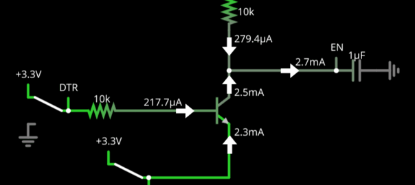
First, we flip the RTS switch. This results in DTR having a higher electrical potential than RTS, and thus some current flowing from the base (B) to the emitter (E). The transistor itself lowers the potential by about 0.6V, so the current coming from B is about (3.3V – 0.6V) / 10kΩ = 270µA.

Since the potential on the base is high, the transistor is in “saturation mode”, meaning that it draws current from the collector (C) to the emitter (E). The amount of current from C to E is proportional to the current from B to E, typically with a ratio of 100. Thus, the transistor draws about 27 mA from C. Since there is a resistor between C and the 3.3V rail, but no resistor between C and the capacitor, most of the current is drawn from the capacitor.
After a very short time (~400 µs), the capacitor gets completely discharged. The transistor draws all the current that can come from the 3.3V rail (3.3V / 10kΩ = 330µA), so EN stays at a 0V potential.

Now, when we flip the DTR switch, E and B are both at 0V, so the transistor effectively “cuts off”. The current from the 3.3V is not drawn by the transistor and instead goes to the capacitor, slowly charging it:

This corresponds to the slow rise of EN, with a characteristic time τ = 10kΩ × 1μF = 10ms. If we flip RTS, the transistor is still in cut-off mode, so this changes nothing.
However, if we also flip DTR, B is now at a higher electrical level than E, putting the transistor into “reverse active” mode. Although this is not the typical way that transistors are used, this is a real phenomenon. As a result, the transistor draws current from E to C!

With DTR at 3.3V and EN at 0V, and considering the ~0.6V voltage drop from the transistor, the base would again draw about 270 µA. However, the capacitor already partially charged from the earlier situation, so the voltage difference between B and C is lower than 3.3V. As a result, we observe a lower current on B (which keeps decreasing).
The gain in reverse active mode is typically lower than in forward active mode. Since this is rarely used, anyway, simulations might not be accurate. To reproduce the observed behavior in CircuitJS, I had to use a gain of 10 instead of the default transistor model with a gain of 1.
In any case, this results in about an additional 2.5mA charging the capacitor, or an almost 10× faster charge! This is exactly what we observe:

This entirely explains the behavior of EN in the breadboard circuit.
Double charged
However, this still does not explain the difference with the ESP-Prog! As a reminder, this is what EN looks like in the breadboard circuit:
And here in the ESP-Prog + Saola:

From the above screenshot, you could think that we no longer have a difference in charging speed between DTR low and DTR high. However, we can still find it if we expand EN:

By tracking back on the reasoning I followed to build the breadboard circuit, I realized that I made an incorrect assumption. Specifically, when looking at the components connected to CHIP_PU on the Saola board, I assumed that the Saola’s own UART-to-USB adapter would not be driving DTR/RTS, and thus do nothing to CHIP_PU.

To challenge this assumption, I removed the red wire that I used to power the Saola board from the ESP-Prog board, and instead connected it with a USB micro-B cable. I also delayed toggling DTR back to 3.3V, so that I could better see the initial charge pattern of EN.
Doing nothing else, I see the same fast-charge pattern:

Then, I just toggled DTR and RTS on the Saola’s UART-to-USB adapter by simply opening the corresponding device with tio (Linux always toggles DTR & RTS), thus cutting off this second reset mechanism. And, lo and behold, EN now charges slower!

If we look at all channels again, it now looks almost identical to the breadboard circuit.

Except…
Just one more thing
Although EN now looks like we expect, IO0 also changed! Let’s look again at all cases:


What we observe is that, when EN becomes electrically low, IO0 slowly discharges, regardless of DTR/RTS. Note that the reverse is not true: IO0 being low does not force EN low. This is different from what we observed in Reproducing Espressif’s reset circuit.
My understanding is that, when we turn the ESP32-S2 chip, we also turn off the voltage regulator that supplies the 3.3V rail used by the reset circuit (with the pull-up resistor), letting a capacitor connected to IO0 slowly discharge.
This is why you might want to desolder R28 and R29, the two 0Ω resistors: this completely disables the Saola’s automatic reset circuit, stopping it from interfering with the ESP-Prog. And this is exactly why R28 and R29 exist.
The end?
This concludes my investigations of Espressif’s reset circuit, but not of UART! There are still a couple of things I do not completely understand and want to uncover before writing the promised “main” article on UART.