Dynamic Programming is not Black Magic

This year’s Advent of Code has been brutal (compare the stats of 2023 with that of 2022, especially day 1 part 1 vs. day 1 part 2). It included a problem to solve with dynamic programming as soon as day 12, which discouraged some people I know. This specific problem was particularly gnarly for Advent of Code, with multiple special cases to take into account, making it basically intractable if you are not already familiar with dynamic programming.

However, dynamic programming itself is mostly natural when you understand what it does. And many common algorithms are actually just the application of dynamic programming to specific problems, including omnipresent path-finding algorithms such as Dijkstra’s algorithm.

This motivated me to write a gentler introduction and a detailed explanation of solving Day 12.

Let me start with a rant. You can skip to the following section if you want to get to the meat of the article.

The Rant

Software engineering is terrible at naming things.

• “Bootstrap” is an imaged expression to point to the absurdity and impossibility of a task, but it has become synonymous with “start” without providing any additional information, such as “boot a computer”. The illusion that it is actually meaningful had lead to an absurd level of polysemy.
• “Daemon”, for a process that is detached from your terminal
• “Cascading Style Sheets”, just to mean that properties can be overridden
• “Cookie”, for a piece of data stored on the Web browser, which is automatically sent to the server
• “Artificial Intelligence” which is so vague it refers just as well to if-conditions, or to AGI

Now, let’s take a look at “dynamic programming”. What can we learn from the name? “Programming” must refer to a style of programming, such as “functional programming”, or maybe “test-driven development”. Then, “dynamic” could mean:

• like in dynamic typing, maybe it could refer to the more general idea of handling objects of arbitrary types, with techniques such as virtual classes, trait objects, or a base Object type.
• maybe it could be the opposite of preferring immutable state
• if it’s not about data, maybe it could be about dynamic code, such as self-modifying code, or JIT
• maybe it could be yet another framework such as Agile, SCRUM, XP, V-model, RTE, RAD
• maybe it could be referring to using practices from competitive programming? Yes, it’s a stretch, but that might make sense

Guess what. It means nothing of that, and it has nothing to do with being “dynamic”. It is an idea that you can use to design an algorithm, so there is a link to “programming”; I will grant it that.

Edit: There is a reason why it is named this way. When you look at the historical meaning of “programming”, the expression made sense. See niconiconi’s comment.

So, what is it?

Basic Caching

Let’s say we want to solve a problem by splitting it in smaller similar problems. Basically, a recursive function. Often, we end-up having to solve the same smaller problems many times.

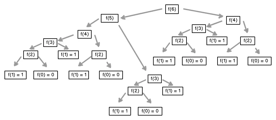
The typical example is Fibonacci, where you want to evaluate f(n), which is defined as f(n - 1) + f(n - 2). If we implement it naively, we will end up evaluating f(1) many times:

In fact, in this case, since only f(1) adds anything to the overall result, the number of times we will need f(1) is equal to f(n). And f(n) grows very fast as n grows.

Of course, we can avoid doing this. We can just cache the results (or memoize f, in terrible academic vernacular).

In the example, once we have evaluated f(4) once, there is no need to evaluate it again, saving 3 evaluations of f(1). By doing the same for f(3) and f(2), we get down to 2 evaluations of f(1). In total, f(…) is evaluated 7 times (f(0), f(1), f(2), f(3), f(4), f(5), f(6)), which is just f(n) + 1.

This is theoretically (asymptotically) optimal. But we can look at this in a different way.

Optimized Caching

With memoization, we keep the recursion: “to solve f(6), I need f(5), which will itself need f(4) […] and f(3) […], and f(4), which will itself need f(3) […] and f(2) […].”. Basically, we figure out what we need just when we need them.

Instead, we can make the simple observation that we will need f(0) and f(1) for all other evaluations of f(…). Once we have them, we can evaluate f(2), which will need for all other evaluations of f(…).

You can think of it as plucking the leaves (the nodes without descendants) from the call tree we saw before, and repeat until there are no more nodes. In other words, perform a topological sort.

With the example, if we have some array F where we can store our partial results:

• F[0] = f(0) = 0
• F[1] = f(1) = 1
• F[2] = f(2) = f(1) + f(0) = F[1] + F[0] = 1 + 0 = 1
• F[3] = f(3) = f(2) + f(1) = F[2] + F[1] = 1 + 1 = 2
• F[4] = f(4) = f(3) + f(2) = F[3] + F[2] = 2 + 1 = 3
• F[5] = f(5) = f(4) + f(3) = F[4] + F[3] = 3 + 2 = 5
• F[6] = f(6) = f(5) + f(4) = F[5] + F[4] = 5 + 3 = 8

With this approach, we do not have any recursive call anymore. And that is dynamic programming.

It also forces us to think clearly about what information we will be storing. In fact, in the case of Fibonacci we can notice that we only need the two last previous values. In other words:

• F[0] = f(0) = 0
• F[1] = f(1) = 1
• F[2] = f(2) = previous + previous_previous = 1 + 0 = 1
• F[3] = f(3) = previous + previous_previous = 1 + 1 = 2
• F[4] = f(4) = previous + previous_previous = 2 + 1 = 3
• F[5] = f(5) = previous + previous_previous = 3 + 2 = 5
• F[6] = f(6) = previous + previous_previous = 5 + 3 = 8

So, we can discard other values and just keep two of them. Doing this in Python, we get:

def fibo(n):
    if n == 0:
        return 0
    previous_previous = 0
    previous = 1
    for _ in range(n - 1):
        current = previous_previous + previous
        (previous, previous_previous) = (current, previous)
    return previous

I like that this gives us a natural and systematic progression from the mathematical definition of the Fibonacci function, to the iterative implementation (not the optimal one, though).

Now, Fibonacci is more of a toy example. Let’s have a look at

Edit Distance

The edit distance between two strings is the smallest number of edits needed to transform one string into the other one.

There are actually several versions, depending on what you count as an “edit”. For instance, if you only allow replacing a character by another, you get Hamming distance; evaluating the Hamming distance between two strings is algorithmically very simple.

Things become more interesting if you allow insertion and deletion of characters as well. This is the Levenstein distance. Considering this title of the present article, this is of course something that can be solved efficiently using ✨ dynamic programming ✨.

To do that, we’ll need to find how we can derive a full solution from solutions to smaller-problems. Let’s say we have two strings: A and B. We’ll note d(X, Y) the edit distance between strings X and Y, and we’ll note x the length of string X. We need to formulate d(A, B) from any combination of d(X, Y) where X is a substring of A and Y a substring of B¹.

We’re going to look at a single character. We’ll use the last one. The first one would work just as well but using a middle one would not be as convenient. So, let’s look at A[a – 1] and B[b – 1] (using zero-indexing). We have four cases:

• A[a - 1] == B[b - 1], then we can ignore that character and look at the rest, so d(A, B) = d(A[0..a - 1], B[0..b - 1])
• A[a - 1] != B[b - 1], then we could apply any of the three rules. Since we want the smallest number of edits, we’ll need to select the smallest value given by applying each rule:
  • substitute the last character of A by that of B, in which case d(A, B) = d(A[0..a - 1], B[0..b - 1]) + 1
  • delete the last character of A, in which case d(A, B) = d(A[0..a - 1], B) + 1
  • insert the last character of B, in which case d(A, B) = d(A, B[0..b - 1]) + 1
• A is actually empty (a = 0), then we need to insert all characters from B², so d(A, B) = b
• B is actually empty (b = 0), then we need to delete all characters from A, so d(A, B) = a

By translating this directly to Python, we get:

def levenstein(A: str, B: str) -> int:
    a = len(A)
    b = len(B)
    if a == 0:
        return b
    elif b == 0:
        return a
    elif A[a - 1] == B[b - 1]:
        return levenstein(A[:a - 1], B[:b - 1])
    else:
        return min([
            levenstein(A[:a - 1], B[:b - 1]) + 1,
            levenstein(A[:a - 1], B) + 1,
            levenstein(A, B[:b - 1]) + 1,
        ])


assert levenstein("", "puppy") == 5
assert levenstein("kitten", "sitting") == 3
assert levenstein("uninformed", "uniformed") == 1
# way too slow!
# assert levenstein("pneumonoultramicroscopicsilicovolcanoconiosis", "sisoinoconaclovociliscipocsorcimartluonomuenp") == 36

As hinted by the last test, this version becomes very slow when comparing long strings with lots of differences. In Fibonnacci, we were doubling the number of instances for each level in the call tree; here, we are tripling it!

In Python, we can easily apply memoization:

from functools import cache

@cache
def levenstein(A: str, B: str) -> int:
    a = len(A)
    b = len(B)
    if a == 0:
        return b
    elif b == 0:
        return a
    elif A[a - 1] == B[b - 1]:
        return levenstein(A[:a - 1], B[:b - 1])
    else:
        return min([
            levenstein(A[:a - 1], B[:b - 1]) + 1,
            levenstein(A[:a - 1], B) + 1,
            levenstein(A, B[:b - 1]) + 1,
        ])


assert levenstein("", "puppy") == 5
assert levenstein("kitten", "sitting") == 3
assert levenstein("uninformed", "uniformed") == 1
# instantaneous!
assert levenstein("pneumonoultramicroscopicsilicovolcanoconiosis", "sisoinoconaclovociliscipocsorcimartluonomuenp") == 36

Now, there is something that makes the code nicer, and more performant, but it is not technically necessary. The trick is that we do not actually need to create new strings in our recursive functions. We can just pass arounds the lengths of the substrings, and always refer to the original strings A and B. Then, our code becomes:

from functools import cache

def levenstein(A: str, B: str) -> int:
    @cache
    def aux(a: int, b: int) -> int:
        if a == 0:
            return b
        elif b == 0:
            return a
        elif A[a - 1] == B[b - 1]:
            return aux(a - 1, b - 1)
        else:
            return min([
                aux(a - 1, b - 1) + 1,
                aux(a - 1, b) + 1,
                aux(a, b - 1) + 1,
            ])
    return aux(len(A), len(B))


assert levenstein("", "puppy") == 5
assert levenstein("kitten", "sitting") == 3
assert levenstein("uninformed", "uniformed") == 1
# instantaneous!
assert levenstein("pneumonoultramicroscopicsilicovolcanoconiosis", "sisoinoconaclovociliscipocsorcimartluonomuenp") == 36

The next step is to build the cache ourselves:

def levenstein(A: str, B: str) -> int:
    # cache[a][b] = levenstein(A[:a], B[:b])
    # note the + 1 so that we can actually do cache[len(A)][len(B)]
    # the list comprehension ensures we create independent rows, not references to the same one
    cache = [[None] * (len(B) + 1) for _ in range(len(A) + 1)]
    def aux(a: int, b: int) -> int:
        if cache[a][b] == None:
            if a == 0:
                cache[a][b] = b
            elif b == 0:
                cache[a][b] = a
            elif A[a - 1] == B[b - 1]:
                cache[a][b] = aux(a - 1, b - 1)
            else:
                cache[a][b] = min([
                    aux(a - 1, b - 1) + 1,
                    aux(a - 1, b) + 1,
                    aux(a, b - 1) + 1,
                ])
        return cache[a][b]
    return aux(len(A), len(B))


assert levenstein("", "puppy") == 5
assert levenstein("kitten", "sitting") == 3
assert levenstein("uninformed", "uniformed") == 1
# instantaneous!
assert levenstein("pneumonoultramicroscopicsilicovolcanoconiosis", "sisoinoconaclovociliscipocsorcimartluonomuenp") == 36

The last thing we need to do is to replace the recursion with iterations. The important thing is to make sure we do that in the right order³:

def levenstein(A: str, B: str) -> int:
    # cache[a][b] = levenstein(A[:a], B[:b])
    # note the + 1 so that we can actually do cache[len(A)][len(B)]
    # the list comprehension ensures we create independent rows, not references to the same one
    cache = [[None] * (len(B) + 1) for _ in range(len(A) + 1)]
    for a in range(0, len(A) + 1):
        for b in range(0, len(B) + 1):
            if a == 0:
                cache[a][b] = b
            elif b == 0:
                cache[a][b] = a
            elif A[a - 1] == B[b - 1]:
                # since we are at row a, we have already filled in row a - 1
                cache[a][b] = cache[a - 1][b - 1]
            else:
                cache[a][b] = min([
                    # since we are at row a, we have already filled in row a - 1
                    cache[a - 1][b - 1] + 1,
                    # since we are at row a, we have already filled in row a - 1
                    cache[a - 1][b] + 1,
                    # since we are at column b, we have already filled column b - 1
                    cache[a][b - 1] + 1,
                ])
    return cache[len(A)][len(B)]


assert levenstein("", "puppy") == 5
assert levenstein("kitten", "sitting") == 3
assert levenstein("uninformed", "uniformed") == 1
# instantaneous!
assert levenstein("pneumonoultramicroscopicsilicovolcanoconiosis", "sisoinoconaclovociliscipocsorcimartluonomuenp") == 36

Now, if you really want to grok dynamic programming, I invite you to try it yourself on the following problems, preferrably in this order:

1. longest common subsequence (not to be confused with longest common substring, but you can do that one too with dynamic programming)
2. line wrap
3. subset sum
4. partition
5. knapsack

Once you are comfortable with dynamic programming, Day 12 should become much less daunting!

Advent of Code, Day 12

In the Advent of Code of December 12th, 2023, you have to solve 1D nonograms. Rather than rephrasing the problem, I will let you read the official description.

.??..??...?##. 1,1,3

This can be solved by brute-force. The proper technique for that is backtracking, another terrible name. But the asymptotic complexity is exponential (for n question marks, we have to evaluate 2ⁿ potential solutions). Let’s see how it goes with this example:

• .??..??...?##. 1,1,3 the first question mark could be either a . or a #; in the second case, we “consume” the first group of size 1, and the second question mark has to be a .
  1. ..?..??...?##. 1,1,3 the next question mark could be either a . or a #; in the second case, we “consume” the first group of size 1, and the next character has to be a ., which is the case
     1. .....??...?##. 1,1,3 the backtracking algorithm will continue to explore the 8 cases, but none of them is a valid solution
     2. ..#..??...?##. (1),1,3
        • and so on…
  2. .#...??...?##. (1),1,3
     • and so on…

There are 32 candidates, which would make 63 list items. I’ll spare you that. Instead, I want to draw your attention to the items 2.2 and 2:

• 2.2. ..#..??...?##. (1),1,3
• 2. .#...??...?##. (1),1,3

They are extremely similar. In fact, if we discard the part that has already been accounted for, they are more like:

• 2.2. .??...?##. 1,3
• 2. ..??...?##. 1,3

There is an extra . on the second one, but we can clearly see that it is actually the same problem, and has the same solutions.

In other words, just like with Fibonacci, the total number of cases is huge, but many of them will just be repeats of other ones. So we are going to apply memoization. And then, dynamic programming.

When we implement the “backtracking” algorithm we’ve overviewed above, we get something like this (not my code):

def count_arrangements(conditions, rules):
    if not rules:
        return 0 if "#" in conditions else 1
    if not conditions:
        return 1 if not rules else 0

    result = 0

    if conditions[0] in ".?":
        result += count_arrangements(conditions[1:], rules)
    if conditions[0] in "#?":
        if (
            rules[0] <= len(conditions)
            and "." not in conditions[: rules[0]]
            and (rules[0] == len(conditions) or conditions[rules[0]] != "#")
        ):
            result += count_arrangements(conditions[rules[0] + 1 :], rules[1:])

    return result

Note the program above handles ? by treating it as both . and #. The first case is easy, but the second case need to check that it matches the next rules; and for that, it needs to check that there is a separator afterwards, or the end of the string.

Since it’s Python, to memoize, we just need to add @cache.

To make it dynamic programing, we use the same trick as in the example of the edit distance: we pass the offset in the string, and the offset in the rules as parameters in the recursion. This becomes:

def count_arrangements(conditions, rules):
    @cache
    def aux(i, j):
        if not rules[j:]:
            return 0 if "#" in conditions[i:] else 1
        if not conditions[i:]:
            return 1 if not rules[j:] else 0

        result = 0

        if conditions[i] in ".?":
            result += aux(i + 1, j)
        if conditions[i] in "#?":
            if (
                rules[j] <= len(conditions[i:])
                and "." not in conditions[i:i + rules[j]]
                and (rules[j] == len(conditions[i:]) or conditions[i + rules[j]] != "#")
            ):
                result += aux(i + rules[j] + 1, j + 1)

        return result
    return aux(0, 0)

Then, we implement our own cache and fill it in the right order:

def count_arrangements(conditions, rules):
    cache = [[0] * (len(rules) + 1) for _ in range(len(conditions) + 1)]
    # note that we are in the indices in reverse order here
    for i in reversed(range(0, len(conditions) + 1)):
        for j in reversed(range(0, len(rules) + 1)):
            if not rules[j:]:
                result = 0 if "#" in conditions[i:] else 1
            elif not conditions[i:]:
                result = 1 if not rules[j:] else 0
            else:
                result = 0
                if conditions[i] in ".?":
                    # since we are at row i, we already filled in row i + 1
                    result += cache[i + 1][j]
                if conditions[i] in "#?":
                    if (
                        rules[j] <= len(conditions[i:])
                        and "." not in conditions[i:i + rules[j]]
                    ):
                        if rules[j] == len(conditions[i:]):
                            # since we are at row i, we already filled in row i + rules[j] > i
                            result += cache[i + rules[j]][j + 1]
                        elif conditions[i + rules[j]] != "#":
                            # since we are at row i, we already filled in row i + rules[j] + 1 > i
                            result += cache[i + rules[j] + 1][j + 1]
            cache[i][j] = result
    return cache[0][0]

And, voilà! You can also have a look at a Rust implementation (my code, this time).

Note: In this case, it looks like the dynamic programming version is slower than the memoized one. But that’s probably due to it being written in unoptimized Python.

Note: Independently from using a faster language and micro-optimizations, the dynamic programming version allows us to see that we only need the previous column. Thus, we could replace the 2D array by two 1D arrays (one for the previous column, and one for the column being filled).

Conclusion

I’ll concede that dynamic programming is not trivial. But it is far from being unreachable for most programmers. Being able to understand how to split a problem in smaller problems will enable you to use memoization in various contexts, which is already a huge improvement above a naive implementation.

However, mastering dynamic programming will let us understand a whole class of algorithms, better understand trade-offs, and make other optimizations possible. So, if you have not already done them, I strongly encourage you to practice on these problems:

1. longest common subsequence (not to be confused with longest common substring, but you can do that one too with dynamic programming)
2. line wrap
3. subset sum
4. partition
5. knapsack

And don’t forget to benchmark and profile your code!

---

1. Excluding, of course, d(A, B) itself ↩︎
2. B could be empty as well, in which case we need to insert 0 characters ↩︎
3. Note that we could permute the inner and outer loops as shown below. In this case, it works just as well:
   for b in range(0, len(B) + 1):
for a in range(0, len(A) + 1):
   ↩︎